TL;DR
Four compounding strategies reduce AI inference cost 60–80%: (1) continuous batching lifts GPU utilization 30–40% to 65–80% for −30 to −50% cost; (2) FP16/AWQ precision cuts memory 2–4x for −20 to −50%; (3) multi-layer caching achieves 60–80% hit rates on eligible traffic for −30 to −60% on repeats; (4) multi-provider arbitrage delivers −20 to −40% by routing to cheapest available GPU within latency SLA. Implementation order: audit, batch, quantize, cache, route.
Why Most AI Teams Overspend on Inference
Before solutions, be precise about where overspend lives.
GPU underutilization is the largest single driver. Average GPU utilization across production AI deployments sits 15–30% without continuous batching. Paying for 100% of hardware, using 15–30%. Every dollar above that floor is pure waste.
Inefficient batching compounds the utilization problem. Processing requests individually means GPU constantly starving, then briefly saturated, then idle.
Over-provisioning for peak load sizes infrastructure for a 5% spike, running at 20% utilization for 95% of the time.
Model precision waste — running FP32 where FP16 or INT8 would serve — doubles or quadruples memory and compute with no quality benefit for most production applications.
Strategy 1: Advanced Batching (Immediate 30–50% Cost Reduction)
Continuous batching is the single highest-leverage optimization. Implementation via vLLM is well-documented.
Critical configuration:
- 1
--max-num-batched-tokens: 16,384–32,768 for throughput - 2
--max-num-seqs: 256+ for high concurrency - 3
--enable-prefix-caching: always on for shared system prompts
Dynamic batch sizing adjusts based on traffic — larger batches off-peak, smaller during peak when latency is priority. GPU utilization 20–40% → 65–80%, translating to 30–50% cost reduction.
Strategy 2: Model Precision Optimization (20–50% Additional Reduction)
Most teams know about precision reduction; fewer implement consistently.
FP16 vs FP32: halves memory, roughly doubles throughput in memory-bandwidth-bound ops — which describes most LLM inference. Quality regression is negligible for virtually all text generation, classification, summarization. Should be the default serving precision for every production model.
AWQ INT4: 4x memory reduction vs FP32. Larger batch sizes per GPU, dramatically lower cost-per-token. Quality tradeoff minimal for most production, entirely acceptable for internal tooling and classification.
GPTQ provides alternative INT4 with different tradeoffs. Both worth benchmarking on your specific model.
Strategy 3: Multi-Layer Caching (30–60% on Eligible Traffic)
Inference requests aren't uniformly novel. In most production AI, a significant percentage are repetitive.
Three-layer architecture: exact-match via Redis for identical inputs, semantic similarity via vector DB for equivalent queries, KV cache prefix sharing for shared prefixes.
Cost reduction depends on traffic patterns — apps with high repetition (support, FAQ, code completion) achieve 60–80% hit rates. Diverse-query apps achieve lower but still benefit from prefix sharing.
Implementation cost: 2–4 weeks engineering for combined layers. Reduction compounds with traffic growth.
Strategy 4: Multi-Provider Cost Arbitrage (20–40% Reduction)
GPU pricing varies significantly across providers and time of day. Single-provider infrastructure pays consistent rate. Multi-provider routing exploits price variation continuously.
OneInfer's Smart Aggregator does this automatically. Configure latency ceiling and cost preference; routing dispatches to cheapest provider meeting latency SLA in real time.
Off-peak: routes to cheaper providers. Peak: shifts to premium maintaining latency. 30-day blended cost reduction: 20–40% vs equivalent single-provider. Combined with prior strategies, cumulative reduction reaches 60–80%.
The Optimization Implementation Order
- 1Audit first. Measure GPU utilization, cost-per-request by model and endpoint, P50/P99 latency. Without baseline, you can't measure progress.
- 2Continuous batching second. Fastest implementation, most immediate impact, no model changes.
- 3Precision third. FP16 everywhere. AWQ where benchmarking confirms acceptability.
- 4Caching fourth. Start with exact-match Redis. Simplest, most obvious wins.
- 5Multi-provider routing last. Integrate OneInfer's unified API; cost-optimized routing operates continuously.
Teams achieving 80% reduction aren't the most sophisticated — they're the ones that implemented these four strategies in sequence, measured each, and kept the optimization compound running. Get in touch with OneInfer.
Run multimodal AI inference at production scale
OneInfer routes every request to the optimal GPU across multiple cloud providers in real time, with sub-500ms latency, AI-generated kernel optimization, and transparent pricing.
Frequently asked questions
+Can I really cut AI inference costs by 80%?
Yes — for most production AI teams. Combining continuous batching (−30 to −50%), FP16/AWQ precision (−20 to −50%), multi-layer caching (−30 to −60% on eligible traffic), and multi-provider arbitrage (−20 to −40%) produces compounding reductions that reach 60–80% in practice.
+What's the single highest-impact AI cost optimization?
Continuous batching. It lifts GPU utilization from typical 20–40% to 65–80% — roughly halving real cost-per-request — with no model changes, no hardware changes, and minimal implementation time using vLLM.
+Should I use FP16 by default for production inference?
Yes. FP16 halves memory and roughly doubles throughput with negligible quality regression for virtually all production text tasks. It should be the default serving precision, not an optimization you evaluate case by case.
+How effective is caching for AI inference?
Three-layer caching (exact-match Redis, semantic similarity, KV prefix sharing) achieves 60–80% hit rates on production traffic for most applications with repeated queries — serving the majority of requests at microsecond latency at near-zero compute cost.
+In what order should I implement AI cost optimizations?
Audit first, then continuous batching, then FP16/AWQ precision, then caching (exact-match first), then multi-provider routing. This sequence delivers compounding gains and lets you measure each step's impact.